Trajectory

noctiluca is intended to facilitate handling and analysis of single (or multi-) particle tracking trajectories. The centerpiece is the Trajectory class; let’s see how to use it.

import numpy as np
from matplotlib import pyplot as plt

import noctiluca as nl

Getting started

At its very core, a Trajectory object is similar to a numpy array. As such, it can be initialized simply from raw data:

traj = nl.Trajectory([1, 0.5, np.nan, 5.4, -2])
nl.plot.vstime(traj)

plt.title('Example trajectory')
plt.xlabel('time [frames]')
plt.show()

Note that we specified a single list of data points. What if we have a 2D trajectory?

Usual SPT trajectories will consist of multiple spatial (xyz) coordinates for a particle. In some cases there might also be multiple particles tracked simultaneously (e.g. multi-color experiments). So in its most general form, a Trajectory has

• \(N\) particles,

• \(T\) frames,

• \(d\) spatial dimensions,

which is represented internally as a numpy array of shape (N, T, d):

print(traj.data.shape)
print(f"N = {traj.N}, T = {traj.T}, d = {traj.d}")

(1, 5, 1)
N = 1, T = 5, d = 1

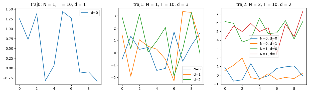
Generally, Trajectory() accepts arrays of shapes (T,), (T, d), or (N, T, d):

traj0 = nl.Trajectory(np.random.normal(size=(10,)))
traj1 = nl.Trajectory(np.random.normal(size=(10, 3)))
traj2 = nl.Trajectory(np.random.normal(size=(2, 10, 2),
                                       loc=[[[0]], [[5]]], # <-- offset to distinguish loci
                                      ))

########## Plotting ############

fig, axs = plt.subplots(1, 3, figsize=[15, 4])

for i, traj in enumerate([traj0, traj1, traj2]):
    ax = axs[i]
    nl.plot.vstime(traj, ax)
    ax.set_title(f"traj{i}: N = {traj.N}, T = {traj.T}, d = {traj.d}")
    ax.legend()

plt.show()

Metadata

Trajectories often carry some annotation, metadata, or other additional information that might be useful. These are stored in the Trajectory.meta dict:

traj = nl.Trajectory([1, 2, 3], comments="This is an example trajectory; not for consumption")
traj.meta['date'] = "2306/07/13"
traj.meta['spot intensity'] = np.array([1.02, 1.5, 0.7])
traj.meta['localization_error'] = np.array([0.5])

print("traj.meta = {")
for key, val in traj.meta.items():
    print(f"    {repr(key):>20s} : {repr(val)}")
print("}")

traj.meta = {
              'comments' : 'This is an example trajectory; not for consumption'
                  'date' : '2306/07/13'
        'spot intensity' : array([1.02, 1.5 , 0.7 ])
    'localization_error' : array([0.5])
}

The entries in this meta-dict can be pretty much anything, whatever you deem useful to know about each trajectory. Note that instead of writing to traj.meta explicitly, you can also provide metadata as keyword arguments to the Trajectory(...) constructor.

Beyond the meta-dict, a Trajectory has two (as of 2022/09/20) additional attributes: localization_error and parity. These are hardcoded to allow propagating them through modifiers; see below.

Modifying trajectories

There are a few common operations that one might want to apply to a trajectory, such as taking an absolute value or calculating an increment trajectory. These are implemented as so-called modifiers:

traj = nl.Trajectory([[1.3, -2], [8.9, 3], [-0.5, 4], [3.2, 1.7]])
abstraj = traj.abs() # takes Euclidean norm --> d = 1
print(f"abstraj.d = {abstraj.d}")
difftraj = traj.diff() # returns increments (like numpy.diff())
traj2 = traj.rescale(1e3) # useful for changing units (e.g. nm <--> μm)

traj = nl.Trajectory(np.random.normal(size=(2, 10, 3)))
reltraj = traj.relative() # returns trajectory of distances between particle 1 and 2
print(f"reltraj.N = {reltraj.N}")

abstraj.d = 1
reltraj.N = 1

A modifier always returns a new trajectory with the given modification applied. By default, metadata is not copied (since it might not apply anymore). To override this, specify the keepmeta keyword argument for any of the above modifiers:

traj = nl.Trajectory([1, -2, 3], mymeta=5)
abstraj = traj.abs()
print(abstraj.meta) # {}

abstraj = traj.abs(keepmeta=['mymeta'])
print(abstraj.meta) # {'mymeta': 5}

{}
{'mymeta': 5}

Missing data

Real data is not perfect; specifically, often there are missing data points. These are specified by np.nan and analysis methods should generally be able to deal with this. It is often useful to know how many frames of a given trajectory are actually valid, i.e. not np.nan; use Trajectory.count_valid_frames() or its alias Trajectory.F (F for “(valid) Frame”).

traj = nl.Trajectory([1, 2, np.nan, 3, np.nan, np.nan, 5])
print(f"valid frames in the trajectory: {traj.count_valid_frames()}")
print(f"                       traj.F = {traj.F}")
print(f"     for reference: len(traj) = {len(traj)} = traj.T")

valid frames in the trajectory: 4
                       traj.F = 4
     for reference: len(traj) = 7 = traj.T

Next: many trajectories

Check out the next example for TaggedSet to learn how noctiluca represents complete datasets containing many individual trajectories. Alternatively, see below for a few more tips and tricks on Trajectory handling. For full reference, always refer to the documentation

Indexing

Trajectories can be indexed along the time dimension using the [] operator, which returns a numpy array:

traj = nl.Trajectory(np.random.normal(size=(2, 10, 3)))
print(f"traj[:].shape  = {traj[:].shape}")
print(f"traj[:7].shape = {traj[:7].shape}")
print(type(traj[:]))

traj[:].shape  = (2, 10, 3)
traj[:7].shape = (2, 7, 3)
<class 'numpy.ndarray'>

The three dimensions of the internal array (N, T, d) may be present or absent in the output, following these rules:

• N is squeezed, i.e. removed if N == 1:

# get a trajectory with N = 1
print(f"traj.relative()[:].shape = {traj.relative()[:].shape}")

traj.relative()[:].shape = (10, 3)

• T follows numpy convention: whether it’s present or not depends on the format of the key:

print(f"traj[:5].shape  = {traj[:5].shape}")
print(f"traj[5].shape   = {traj[5].shape}")
print(f"traj[[5]].shape = {traj[[5]].shape}")

traj[:5].shape  = (2, 5, 3)
traj[5].shape   = (2, 3)
traj[[5]].shape = (2, 1, 3)

• d is always present in the output, even if there is only one spatial dimension. This is such that analysis code can be fully agnostic of spatial dimension; squeezing this last dimension can be done by hand if necessary, as illustrated below

abstraj = traj.abs() # get a trajectory with d = 1
print(f"abstraj[:].shape                  = {abstraj[:].shape}")
print(f"abstraj[:][..., 0].shape          = {abstraj[:][..., 0].shape}")
print(f"abstraj.relative()[:].shape       = {abstraj.relative()[:].shape}")
print(f"abstraj.relative()[:][:, 0].shape = {abstraj.relative()[:][:, 0].shape}")

abstraj[:].shape                  = (2, 10, 1)
abstraj[:][..., 0].shape          = (2, 10)
abstraj.relative()[:].shape       = (10, 1)
abstraj.relative()[:][:, 0].shape = (10,)

Plotting

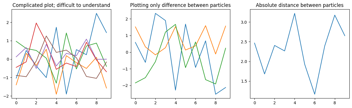
We already saw the nl.plot.vstime() method for plotting a trajectory over time. If you have a complicated trajectory (with multiple particles and/or spatial dimensions), you can use modifiers to simplify plots:

traj = nl.Trajectory(np.random.normal(size=(2, 10, 3)))

fig, axs = plt.subplots(1, 3, figsize=[15, 4])

ax = axs[0]
nl.plot.vstime(traj, ax=ax)
ax.set_title('Complicated plot; difficult to understand')

ax = axs[1]
nl.plot.vstime(traj.relative(), ax=ax)
ax.set_title('Plotting only difference between particles')

ax = axs[2]
nl.plot.vstime(traj.relative().abs(), ax=ax)
ax.set_title('Absolute distance between particles')

plt.show()

If there is no useful simplification to be made to the data before plotting, you can beautify the plot after the fact to make it more digestible. To that end, nl.plot.vstime() returns a list of the lines it adds to the axes, so we can simply adjust their properties. The returned list is sorted by N * d, i.e. [:d] are the spatial dimensions of particle 0, [d:(2*d)] are particle 1, etc.

traj = nl.Trajectory(np.random.normal(size=(2, 10, 3)))

fig, axs = plt.subplots(1, 2, figsize=[10, 4])

ax = axs[0]
nl.plot.vstime(traj, ax=ax)
ax.set_title('Complicated plot; difficult to understand')

ax = axs[1]
lines = nl.plot.vstime(traj, ax=ax)
for i in range(traj.d):
    lines[traj.d+i].set_color(lines[i].get_color())
    lines[traj.d+i].set_linestyle('--')

    lines[i].set_label(f'd={i}')
    lines[traj.d+i].set_label('')

# Add some fake legend entries
ax.plot(np.nan, np.nan, linestyle='-',  color='k', label='N=0')
ax.plot(np.nan, np.nan, linestyle='--', color='k', label='N=1')

ax.set_title('(somewhat) more parseable plot')
ax.legend(loc=(1.02, 0.5))

plt.show()

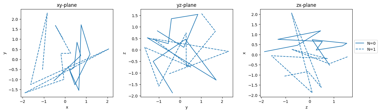
There is another method for visualizing trajectories: nl.plot.spatial() plots a given trajectory in the xy-coordinate plane. For trajectories with more than two spatial dimensions you can specify which dimensions you want to plot:

traj = nl.Trajectory(np.random.normal(size=(2, 10, 3)))

fig, axs = plt.subplots(1, 3,
                        figsize=[15, 4],
                        gridspec_kw={'wspace' : 0.3},
                       )

for i, (ax, dims) in enumerate(zip(axs, [(0, 1), (1, 2), (2, 0)])):
    lines = nl.plot.spatial(traj, ax=ax, dims=dims)
    lines[1].set_color(lines[0].get_color())
    lines[1].set_linestyle('--')

    dims_chr = tuple(chr(ord('x')+d) for d in dims)
    ax.set_title(dims_chr[0]+dims_chr[1]+'-plane')
    ax.set_xlabel(dims_chr[0])
    ax.set_ylabel(dims_chr[1])

axs[-1].legend(loc=(1.02, 0.5))
plt.show()